Module 2: Expressing and Analyzing Algorithms

What Can A Computer Do?

• computers can only perform binary operations that take two operands

  • adding two numbers or

  • multiplying two numbers or

  • comparing two numbers

Finding the Maximum Value

1. remember the largest value you have seen so far starting at the beginning of the list and store it in a variable named max

2. compare it to the next value in the list

3. update the largest value (max) so far

Algorithm: Find-Max

Problem: Find the maximum value in a list of values

• at first, the max is the first one in the list

• look at each value in the list. if it is greater than the current max, then that value becomes the max

• after going through the entire list, the current max is the maximum value in the list

Flowchart: Find-Max

Flowchart: Find-Min

Telling the Computer How to Search

• a computer can't process the list all at once

• it can only compare two things at a time

• the algorithm must be expressed in terms of binary comparisons

Algorithm: Searching for a Value

Problem: Determine whether a list of values contains a target value

• Look at each value in the list. If it is equal to the target, then we have found the value and we can stop looking

• If we go through the entire list and have not found the target, then it is not in the list

Flowchart: Searching for a Value

Improving Search for Ordered Lists

• Any search algorithm must determine where to look first, and then where to look next

• In linear search, we start with the first item and then look at the next item

• What if we were to start with the middle item?

So, just simply ordering the list can cut down on the search time because if you were to search for an item and the current you were on is greater than the target, then you can simply stop your search and know that your target is not in the list. However, is an unordered list and using linear search, then you would need to search through all items to make sure your target was not in the list. So simply ordering the list can cut down on the search time.

In a binary search though, not only is the list ordered, but you move where you begin your search as well. You start with the middle item and determine is this your target, if not, then is it greater than or less than your target. By this determination, you can cut down on the number items left to search in half. You keep doing this until either you find what you are looking for or you don't.

Searching for a Value: Sorted List

[4, 7, 8, 12, 22, 25, 31, 34, 38, 42, 49, 51, 58, 60]

Target: 42 Found: No

[4, 7, 8, 12, 22, 25, *31*, 34, 38, 42, 49, 51, 58, 60]

Target: 42 Found: No

Start with the middle item (31), not found, so is the target greater than or less than?

In this case, it is greater than, so we can eliminate the first half already, no need to search through them.

[4, 7, 8, 12, 22, 25, 31, 34, 38, 42, *49*, 51, 58, 60]

Target: 42 Found: No

Once again, start with the middle term (49), not found, so is the target greater than or less than the current item?

Now it is less than, so we can now eliminate everything beyond the current item. This leaves us just [34, 38, 42] left.

[4, 7, 8, 12, 22, 25, 31, 34, *38*, 42, 49, 51, 58, 60]

Target: 42 Found: No

Once again start with the middle term (38), not found, is the target greater than or less than the current item. It is greater, so we just eliminated [34, 38].

[4, 7, 8, 12, 22, 25, 31, 34, 38, *42*, 49, 51, 58, 60]

Target: 42 Found: Yes

So we found our target on the fourth iteration vs. a linear search we would not have found the target until the 11th iteration.

Algorithm: Binary Search

Problem: Determine whether a sorted list of values contains a target value

• Repeat these steps whether a sorted list of values contains a target value

  • Compare the value in the middle fo the list to the target

  • If they are equal, then we have found the target and can stop looking

  • If the value in the middle of the list is greater than the target, remove the middle element and elements that are larger than it and repeat

  • If the value in the middle of the list is less than the target, remove the middle element and elements that are smaller than it and repeat

• If we remove all elements in the list, then it does not contain the target

Flowchart: Binary Search

Binary Search: Complexity

Using the above list again and now a target value is not in the list (worst case scenario), it would still only take 4 comparisons before we eliminated all elements and determined the value is not in the list using the Binary Search Algorithm.

The worst case scenario using linear search would take 15 comparisons before reaching the same conclusion.

To describe the complexity, let's double the list size and evaluate the number of comparisons. This would only increase the number of comparisons by one from the original list.

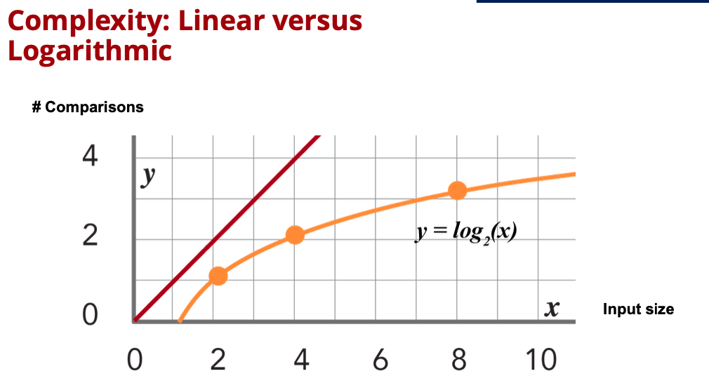
Here the linear search complexity is shown in red, and the binary search is shown in orange. So, as the number of inputs increases, the linear search number of comparisons also increases at the same rate. But, notice the binary search does not; it eventually gets to a point where you increase the number of inputs and no appreciable increase in the number of comparisons. This is known as logarithmic complexity. The number of comparisons grows at the rate of the logarithm of the number of inputs increases.

Finding the Maximum Value

How many comparisons were needed to find the max value?

[*52.3*, 81.2, 33.6, 17.3, 25.1, 90.4, 28.2, 43.1]

• first value = max and

• no. of comparisons 0

[-52.3-, *81.2*, 33.6, 17.3, 25.1, 90.4, 28.2, 43.1]

• second value compared to max - largest so far is 81.2 and

• no. of comparisons 1

[52.3, -81.2-, *33.6*, 17.3, 25.1, 90.4, 28.2, 43.1]

• third value compared to max - largest so far 81.2 and

• no. of comparisons 2

[52.3, -81.2-, 33.6, *17.3*, 25.1, 90.4, 28.2, 43.1]

• fourth value compared to max - largest so far 81.2 and

• no. of comparisons 3

[52.3, -81.2-, 33.6, 17.3, *25.1*, 90.4, 28.2, 43.1]

• fifth value compared to max - largest so far 81.2 and

• no. of comparisons 4

[52.3, -81.2-, 33.6, 17.3, 25.1, *90.4*, 28.2, 43.1]

• sixth value compared to max - largest so far 90.4 and

• no. of comparisons 5

[52.3, 81.2, 33.6, 17.3, 25.1, -90.4-, *28.2*, 43.1]

• seventh value compared to max - largest so far 90.4 and

• no. of comparisons 6

[52.3, 81.2, 33.6, 17.3, 25.1, -90.4-, 28.2, *43.1*]

• seventh value compared to max - largest so far 90.4 and

• no. of comparisons: 7

[52.3, 81.2, 33.6, 17.3, 25.1, -90.4-, 28.2, 43.1]

• largest so far 90.4 and

• no. of comparisons = no. of elements - 1

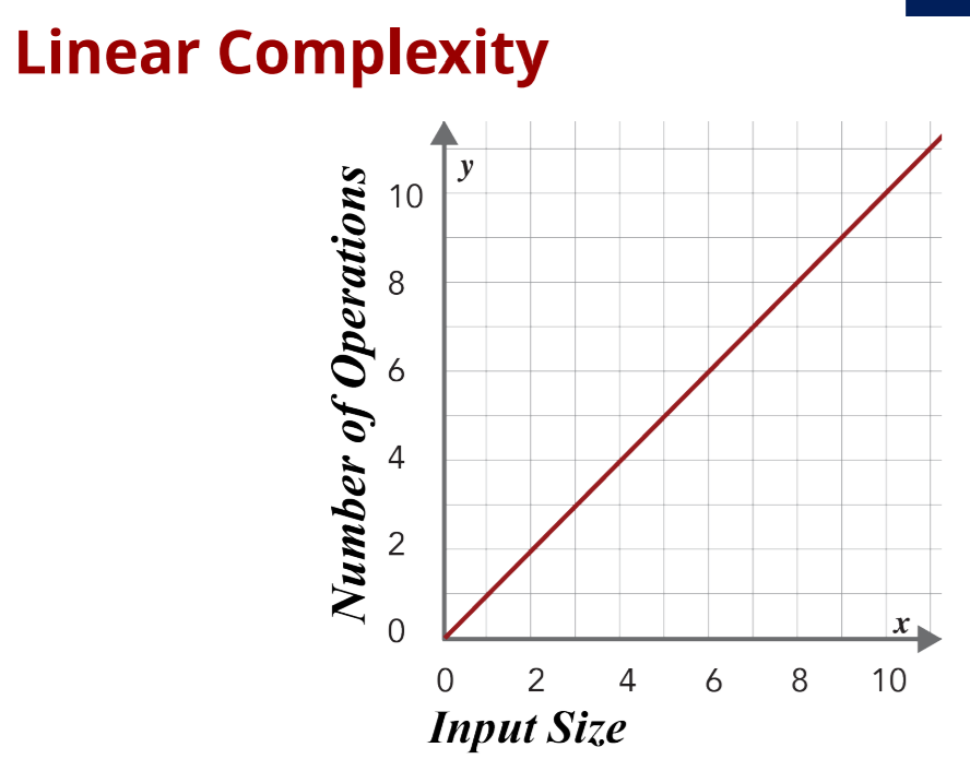
If we double the number of elements, we still must compare against all them. This would result in a total of 15 comparisons which is again no. Of elements - 1. What this boils down to is if we double the number of elements, then we also double the number of comparisons and so on. This is called linear growth. The number of comparisons roughly equals the number of elements. This algorithm has linear complexity.

Searching for a Value

[52.3, 81.2, 33.6, 17.3, 25.1, 90.4, 28.2, 43.1]

• Target: 90.4

• Found: No

• No. of Comparisons: 0

[*52.3*, 81.2, 33.6, 17.3, 25.1, 90.4, 28.2, 43.1]

• Target: 90.4

• Found: No

• No. of Comparisons: 1

[52.3, *81.2*, 33.6, 17.3, 25.1, 90.4, 28.2, 43.1]

• Target: 90.4

• Found: No

• No. of Comparisons: 2

[52.3, 81.2, *33.6*, 17.3, 25.1, 90.4, 28.2, 43.1]

• Target: 90.4

• Found: No

• No. of Comparisons: 3

[52.3, 81.2, 33.6, *17.3*, 25.1, 90.4, 28.2, 43.1]

• Target: 90.4

• Found: No

• No. of Comparisons: 4

[52.3, 81.2, 33.6, 17.3,* 25.1*, 90.4, 28.2, 43.1]

• Target: 90.4

• Found: No

• No. of Comparisons: 5

[52.3,*81.2, 33.6, 17.3, 25.1,* 90.4*, 28.2, 43.1]

• Target: 90.4

• Found: Yes

• No. of Comparisons: 6

Assuming 90.4 stays in the same place, and we double the number of inputs, it would still only take 6 comparisons. The number of elements that come after really does not matter, therefore doubling the number of elements really does not take any more time than before.

But when we analyze the complexity of an algorithm, we use the worst case to give up a better idea of what might happen when the number of elements grows.

Now, let's try a search where the target is not within the list. We have to look at every element in the list.

[52.3, 81.2, 33.6, 17.3, 25.1, 90.4, 28.2, 43.1]

• Target: 50.5

• Found: No

• No. of Comparisons: 0

[*52.3*, 81.2, 33.6, 17.3, 25.1, 90.4, 28.2, 43.1]

• Target: 50.5

• Found: No

• No. of Comparisons: 1

[52.3, *81.2*, 33.6, 17.3, 25.1, 90.4, 28.2, 43.1]

• Target: 50.5

• Found: No

• No. of Comparisons: 2

[52.3, 81.2, *33.6*, 17.3, 25.1, 90.4, 28.2, 43.1]

• Target: 50.5

• Found: No

• No. of Comparisons: 3

[52.3, 81.2, 33.6, *17.3*, 25.1, 90.4, 28.2, 43.1]

• Target: 50.5

• Found: No

• No. of Comparisons: 4

[52.3, 81.2, 33.6, 17.3, *25.1*, 90.4, 28.2, 43.1]

• Target: 50.5

• Found: No

• No. of Comparisons: 5

[52.3, 81.2, 33.6, 17.3, 25.1, *90.4*, 28.2, 43.1]

• Target: 50.5

• Found: No

• No. of Comparisons: 6

[52.3, 81.2, 33.6, 17.3, 25.1, 90.4, *28.2*, 43.1]

• Target: 50.5

• Found: No

• No. of Comparisons: 7

[52.3, 81.2, 33.6, 17.3, 25.1, 90.4, 28.2, *43.1*]

• Target: 50.5

• Found: No

• No. of Comparisons: 8

Now, if we double the number of elements, then we also roughly double the number of comparisons we have to do. This is still linear and therefore linear complexity.

Example 1

Problem: I love to go there and always want to see as many exhibits and attend as many events as possible, but we can only make it one day a month, and sometimes exhibits and events are only held on different days of the week or in different months. So, figuring out which day we should go each month is an optimization problem. We want to figure out on which day we should go each month so that we can do as many different things as possible.

Data: January - 21, 22; February - 11,18, 25, 26, 27; March - 3, 10, 11, 12; April - 12, 19, 26

Brute Force: choose one day from each of the four months adn then figure out how many different exhibits I'll be able to see using that combination of visits. I can do this for all possible combinations of days. Once I've looked at all those possible solutions, I can choose the one that allows me to see and do the most things at the museum.

One solution is: Jan 22, Feb 18, Mar 11, Apr 12

How many ways are there to choose one day from each month? Look at the months of January and February

• there are two days in January and 5 days in February, so 2 * 5 = 10 (multiply the number of individual options). There are 10 possible combinations of days

• now adding March for each of those 10 possibilities, there are four days possible in March. Now, we have 10 * 4 = 40

• now adding in April, for each of the 40 possible combinations there 3 days in April, so 40 * 3 = 120

Therefore, I can look at all 120 combinations and find the one that allows me to see the most exhibits. Although this approach would definitely work, that is a lot of combinations to consider.

Example 2

Problem: Need to meet with 8 TAs at least once per week. Available times to meet with each TA based on my schedule comes out to certain times Mon-Thurs. I also want to minimize the number of meetings. So, there are two out comes for each time. I can either include it or not include it.

Data: Mon - 16:00, Tues = 18:00, Wed - 13:00, Wed - 16:00, Thurs - 18:00

So, once again there 2 options for each time above and 5 times total. This is 2 x 2 x 2 x 2 x 2 = 32 (2**5).

Brute force has exponential complexity. For every additional time added, the number of possible combinations doubles.

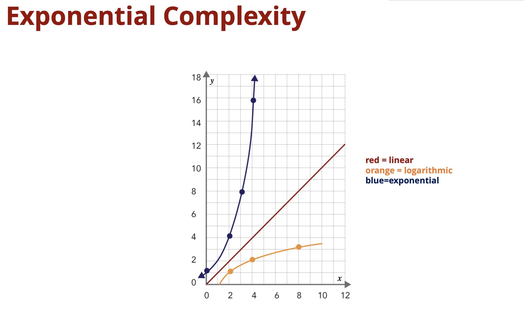
Although this seems bad, for some problems, this is maybe the only way to get at the solution. And sometimes, it may even grow faster than exponentially.

Example 3

Problem: Determine the shortest path. Starting from a single mulch pile you have a yard with eight flower beds that need mulch. You need to mulch all eight beds, and you need to do this with the least amount of walking in between those beds.

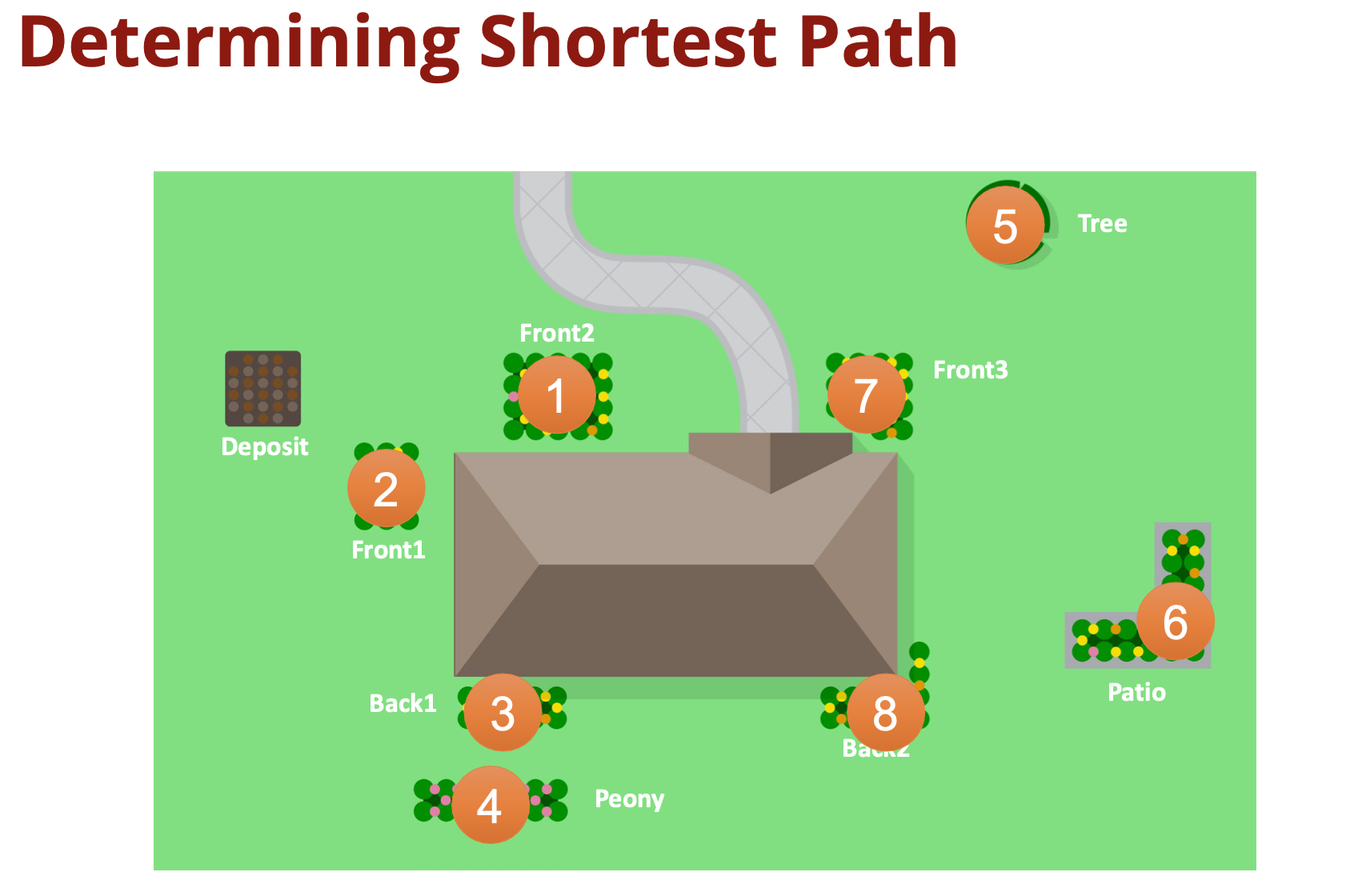
So, what's the best route for you to take? One way we can solve this problem is by looking at all the possible routes between the flower beds and then finding the one that's shortest. So, how many possible routes are there? Well, a route here is a sequence of the eight locations where the order matters. Each route is a possible solution to this problem. When the order matters, we say that this is a permutation. So, how many different permutations of those eight things exist? So, as I said, you have to start at the mulch deposit, and then from here, there are eight places where you can go. That is, each of the eight different flowerbeds. Let's say that from the deposit, you decide to go to the tree first. After the tree, now there are seven places where you can go for the second flower bed. Regardless of which one of the eight you picked as the first flowerbed, after that there are seven possible places to go for the second, because you can't go back to the mulch deposit yet, and you can't stay where you are. So, now let's say that after the deposit and then the tree, you'd go to the patio next. After that, now you have six different flower beds to choose from since you can't go back to one of the two you have already done, and you're not finished yet. So, regardless of which of the seven, you picked for the second flowerbed, there are six possible flower beds for the third and so on.

So, how many possible solutions are there? Well, for the first flowerbed, there are eight possible options. For the second choice, there are seven. For the third, there are six and so on. This gives us a total of 40,320 different possible routes through the eight flower beds (8!).

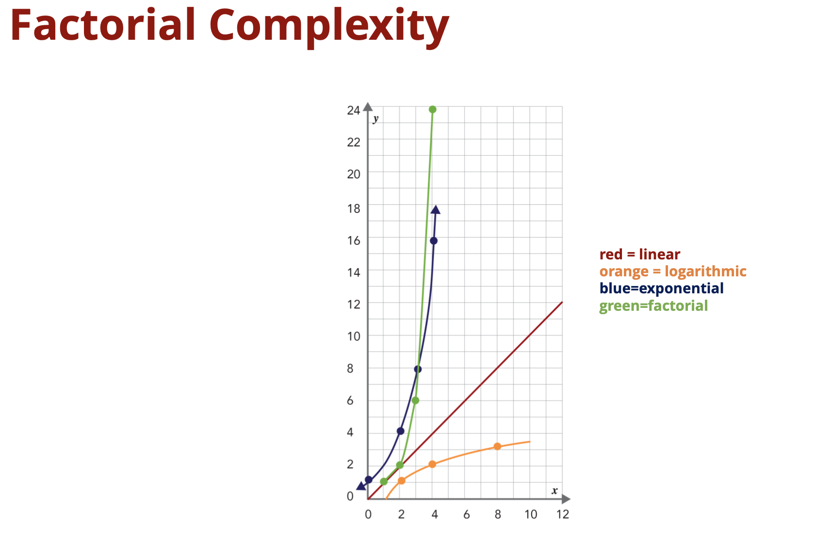
Another flowerbed is added to your garden and now instead we have nine options. How many permutations would there be now? Well, if we increase it by one to nine options, then we'd have nine factorial possible solutions or permutations. That's nine times eight times seven times six and so on, and this is over 360,000 (9!) possible paths through the garden. This approach exhibits factorial complexity.

Summary

• Brute force algorithms can be used for solving optimization problems

  • try all possible solutions

  • identify the ones that solve the problem

  • determine the one that is best

• There can be many solutions

• For an input of n elements:

  • Exponential complexity: 2n possible solutions

  • Factorial complexity: n! possible solutions